Effect of initial estimates for KLLs on the convergence of liquid-liquid equilibrium calculations

The initial estimates for the KLLs (equilibrium factors) have a big influence on the convergence behavior of liquid-liquid equilibrium calculations.

To highlight this effect, let’s try out something with LIBPF.

We choose the system H2O / 2-ethyl-1-hexanol.

Experimental measurements for the liquid-liquid equilibrium of this system can be found in the publication: Frank Gremer, Gerhard Herres, Dieter Gorenflo, “Vapour – liquid and liquid – liquid equilibria of mixtures of water and alcohols: measurements and correlations“, High Temperatures – High Pressures, 2002, volume 34, pages 355 – 362 (direct link). We are also grateful to the authors for providing additional data.

Let’s pick from from that source the data point at 120.384 – 129.785°C, here are the water molar fraction:

• watery phase 0.9998 mol/mol
• organic phase 0.334 mol/mol

Fitting this data-point we get these NRTL binary parameters:

• alfa = 0.2
• B12 = 3060.4764877456
• B21 = -156.0296483827

These parameters can be used to reproduce the chosen experimental data point, see the HOWTO calculate a liquid-liquid separation tutorial.

The program yields these results:

------------------------------------------------------------------------------------
Phase   fraction        Water   ETEX    Water   ETEX
Name    mol frac        mol frac        ndot, kmol/s    ndot, kmol/s
STREAM:Vphase   0.278635989043  0.999484893116  0.000515106883773       27.8492 0.0143527
STREAM:Lphase   0.721364010957  0.30706763201   0.69293236799   22.1508 49.9856
STREAM:Tphase   1       0.5     0.5     50      50
------------------------------------------------------------------------------------
Water Kll: 3.25493405663 
ETEX Kll:  0.000743372524604

Here Vphase is the first liquid phase, and Lphase is the second liquid phase.

We have used KLL[0] = 1E5 and KLL1 = 1E-5 as initial estimates, making the first component (the water) more affine with the first liquid phase. Consequently the solver converges to a solution (let’s call it solution B) where the organic phase is the second liquid phase.

If we set each KLL to its reverse (1E-5 and 1E5 respectively) we get the same results, but the phases are inverted:

------------------------------------------------------------------------------------
Phase   fraction        Water   ETEX    Water   ETEX
Name    mol frac        mol frac        ndot, kmol/s    ndot, kmol/s
STREAM:Vphase   0.721364010957  0.30706763201   0.69293236799   22.1508 49.9856
STREAM:Lphase   0.278635989043  0.999484893116  0.000515106883773       27.8492 0.0143527
STREAM:Tphase   1       0.5     0.5     50      50
------------------------------------------------------------------------------------
Water Kll: 0.307225886179 
ETEX Kll:  1345.22055484

here the organic phase is the first phase (let’s call it solution A) and the final KLLs are the reciprocal of those in solution B !

Now let’s try a scan of the range of possible initial estimates for the KLLs, sweeping each from 1E-5 to 1E5:

std::cout << "kll0\tkll1\terrors\titerations\tVphase.x[0]\tLphase.x[0]" << std::endl;
double factor(10.0);
for (double kll0=1E-5; kll0<1E5; kll0*=factor) {
  for (double kll1=1E-5; kll1setPristineRecursive();
    feed->resetErrors();
    feed->calculate();
    // TODO automate valid initial point table
    std::cout << kll0 << "\t" << kll1 << "\t" <errors.size() << "\t" <NITER_NLEFlash.value() << "\t" <Q("Vphase.x[0]") << "\t" <Q("Lphase.x[0]") << std::endl;
  } // loop over kll1
} // loop over kll0

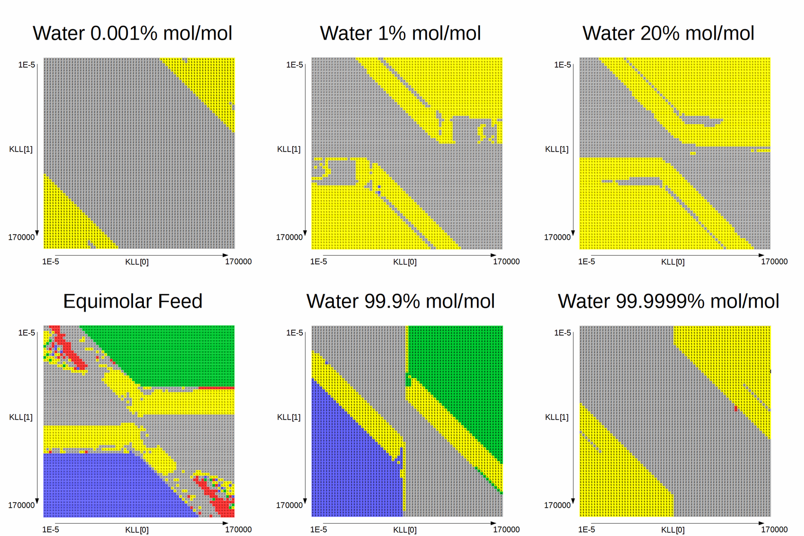
This prints a 10×10 grid which looks like this:

kll0    kll1    errors  iterations      Vphase.x[0]     Lphase.x[0]

1e-05   1e-05   0       1       0.5     0.5 
1e-05   0.0001  2       500     0.454166789146  0.5 
...
1e-05	10000	0	4	0.143450341144 	0.999719891117 
...
10000	1e-05	0	4	0.999719891047 	0.143450278799 
...

There are four possible situations:

1. the liquid-liquid split is found, with the 1st liquid being the organic phase: solution A
2. the same liquid-liquid split is found, with the 2nd liquid being the organic phase: solution B
3. we have errors: the initial estimate was off and did not enable the nonlinear algebraic solver to find the solution
4. it converges, but the degenerate solution (with both phases having the same composition) is found

We can generate several of these grids, with the water content in the feed spanning the entire range of compositions.

This animated GIF shows a slideshow of the results:

Here the blue color stands for solution A, green for solution B, red for errors, yellow for single-phase and gray for degenerate solution.

We note the following:

1. when the initial estimates for the KLLs are close to one another, the degenerate solution is always found

2. intermediate initial estimates typically cause convergence errors or a spurious single-phase solution

3. if the alcohol fraction is greater than water:

   • if the difference between the initial estimate of the equilibrium factor for the alcohol (KLL1) and the one for the water (45° sloped boundary of the blue area) is higher than a certain difference threshold and the initial estimate of the equilibrium factor for the alcohol (KLL1) is higher than than another threshold, solution A is found
   • the sloped boundary advances to the right (i.e. the maximum difference threshold is decreased) as the water content in the feed increases
   • if the difference between the initial estimate of the equilibrium factor for the alcohol (KLL1) and the one for the water (45° sloped boundary of the blue area) is lower than a certain difference threshold and the one for the alcohol (KLL1) is lower than another threshold, solution B is found
   • the sloped boundary advances to the left (i.e. the maximum difference threshold is decreased) as the water content in the feed increases

4. if the water fraction is greater than alcohol:

   • the shape of the blue / green areas flip
   • the 45° sloped boundaries recede to the bottom / top as the alcohol content in the feed decreases

Conclusions: the initial estimates of the equilibrium factors can be used to steer the solver towards making the first or the second phase the organic phase; for example to make the second phase the organic phase (solution B) a practical initialization strategy is to set the KLLs for the key organic components (those present in large amount) to small value such as 1E-5, and the KLL for for water to a large value such as 1E5. The KLLs for the trace components can be left uninitialized to their default value of 1.