Detailed process model description for the Gas Membrane separation demo
Model specification
Introduction
Intended audience
The present document is oriented to:
-
Model developers
-
Model users
-
System Integrators.
Scope
The scope of the present document is to describe the capabilities of the Gas Membrane separation demo, for the process modeling of gas purification processes based on gas membranes such as biogas upgrading and CO2 postcombustion separation.
Gas mixtures can be separated by compressing and pushing them through a membrane. The chemical components in the mixture typically have different permeabilities, so the fraction that goes through the membrane (the permeate) will be richer than the fraction that does not (the retentate) in the components with higher permeabilities.
Today gas separation membranes find many applications:
- olefin recovery in poly-olefin plants
- gasoline vapors recovery from tank farms and fuel terminals
- VOC (volatile organic component) recovery in refrigerator and process vents
- hydrogen separation
- oxygen–nitrogen separation
- methane purification
- post-combustion carbon dioxide capture.
The separation of carbon dioxide (CO₂) from methane is useful for natural gas processing, biogas purification and upgrading, enhanced oil recovery and flue gas treatment. CO₂ must be removed from natural gas mainly to prevent pipe corrosion and avoid degradation of the heating value.
Recently the separation of CO₂ from the flue gases deriving from the combustion of fossil fuels has gained much attention in the context of greenhouse gases emission reduction.
Finally membrane units can be used for process intensification to decrease production costs but also equipment size, energy utilization, and waste generation.
In general the advantages of gas purification processes based on membranes are:
-
relatively low capital cost
-
equipment simplicity
-
and modularity.
With membranes the driving force for the separation is pressure and the operating costs are controlled by the electrical power consumption of the compressors.
In order to minimize power consumption while at same time ensuring both high recovery and high purity, cascades with multiple membrane stages and recycle streams between the stages are employed.
This demo is focused on biogas upgrading and CO₂ postcombustion separation processes.
Prerequisites
-
basic knowledge of process engineering and / or of gas membrane processes;
-
know about the different roles involved with the lifecycle of solutions developed using the LIBPF® enabling technology, see LIBPF® Technology Introduction.
Gasmem kernel
In LIBPF® one kernel can support many process models, each as a different flowsheet type.
All the process models supported by a kernel share the same list of components and can use all LIBPF® embedded types plus the custom types registered by the kernel itself.
Type list
The Gasmem kernel registers the following models, based on the built-in LIBPF® FlowSheet type:
| Type | Description |
|---|---|
Merkel2010Fig7a |
Post-combustion Co2 capture for power plants Figure 7a of Merkel2010, with free-flow, multi-stage membrane model but without permeate sweep |
Merkel2010Fig7aCounterflow |
Configurable Merkel2010 Figure 7a counter-flow |
Merkel2010Fig7aLinearCounterflow |
Post-combustion CO2 capture for power plants Figure 7a of Merkel2010 with linear average, counter-current, multi-stage membrane model |
Merkel2010Fig7b |
Configurable Merkel2010 Figure 7b |
Merkel2010Fig7bLinearCounterflow |
Post-combustion CO2 capture for power plants Figure 7b of Merkel2010 with linear average, counter-flow/sweep multi-stage membrane model |
Merkel2010Fig11 |
Post-combustion CO2 capture for power plants Figure 11 Merkel2010 (three-step vacuum membrane process) |
Deng2010Fig6b |
Biogas upgrading Figure 6b of Deng2010 (two-step without recycle) |
Makaruk2010Fig2 |
Configurable Makaruk2010 Figure 2: two-step low-pressure-feed cascade |
Makaruk2010Fig2FreeFlowRtsc |
Biogas upgrading Figure 2 of Makaruk2010 (two-step low-pressure-feed cascade), with free flow, multi-stage, RTSC membrane model |
Makaruk2010Fig2FreeFlowCstr |
Biogas upgrading Figure 2 of Makaruk2010 (two-step low-pressure-feed cascade), with free flow, multi-stage, CSTR membrane model |
Benchmark |
Reference biogas plant with Internal Combustion Engine |
Upgrading |
Biogas plant with two-step upgrading |
Component list
The fluids to be processed are broken down in their constituents and represented as a mixture of basic components.
The components are defined using built-in LIBPF® basic types.
More precisely the Gasmem kernel defines the following component list (click on the component type to jump to the reference documentation for the component):
components.addcomp(new purecomps::CO2);
components.addcomp(new purecomps::methane);
components.addcomp(new purecomps::water("H2O"));
components.addcomp(new purecomps::N2);
components.addcomp(new purecomps::O2);
| Type | Name | Description |
|---|---|---|
| purecomps::CO2 | CO2 | standard model for carbon dioxide |
| purecomps::methane | CH4 | standard model for methane |
| purecomps::water | water | standard model for water |
| purecomps::N2 | N2 | standard model for nitrogen |
| purecomps::O2 | O2 | standard model for oxygen |
Process descriptions and schemes
LIBPF® is based on an object-oriented approach (object-oriented) so each real physical entity (object) corresponds to a simulated object instance. What is common to a set of simulated objects can be generalized into a class, which is a model for creating objects.
To make it easier to simulate processes that include gas membranes, a number of low-level models have been prepared, to simulate various membrane types with different modeling approaches.
Low-level models
For example, a model instance of type MembraneMulti12<...> is represented in the figure:
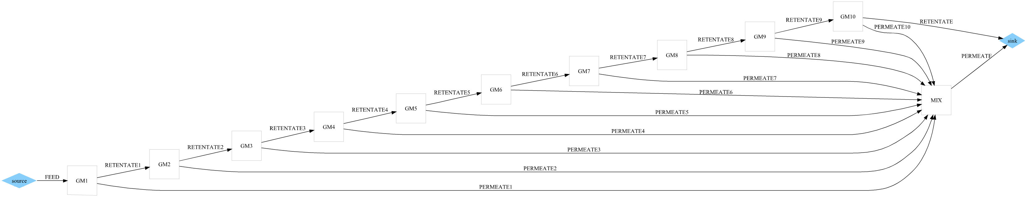
Whereas this is the internal connectivity of a model instance of the type MembraneMulti22...Coflow:

In this case, the permeate of each sub-unit passes to the next sub-unit of which will constitute the permeate sweep. As in modeling in free-flow the retentate of each sub-unit will pass to the next sub-unit as the feed.
Finally this is the internal connectivity of a model instance of the type MembraneMulti22RtscCounterflow:

Unlike the case in co-flow we see that the user-defined permeate sweep enters the last stage (GM10). Compared to the previous cases in co-flow and free-flow we see that in this case, while the final retentate is taken from the last subunit, the permeate is taken from the first.
This implies an additional iteration for convergence of internal recycles.
Membrane12Rtsc
Units with one-two connectivity and global fluid dynamics “RTSC,” is implemented as a class derived from Separator<N>, the model that represents a generic separator with fixed separation yields with
The coefficients outSplit[2][n_c] that are input to the basic model Separator<2> are a matrix of the stage cuts of each component, indexed by the ordinal of the output and the ordinal of the component. The stage cuts must be positive (if negative values are specified, they are considered zero).
The columns of the outSplit matrix must be normalized, that is, for any given component, the sum of the stage cuts of the component to all outputs must be unity. If the user specifies stage cuts toward the first
Consequently, it is preferable to specify already normalized values for all components and for all but the last output.
For the Membrane12Rtsc model, the coefficients outSplit[2][n_c] in the base model Separator<2> are set according to the balances at the membrane.
Connections:
-
feed i.e.
in1 -
permeate i.e.
out1 -
retentate i.e.
out2
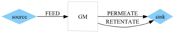
where source and sink are the blocks by which the program acquires input data (source) and returns output data (sink) from the flow-sheet.
Input variables:
permeance[n_c] |
Permeance of each component, corresponds to the variable |
|
Ppermeate |
Permeate compartment pressure | Pa |
deltaPretentate |
Retentate side pressure drop | Pa |
A |
Active area of the membrane | |
Explicit equations (note the expression for outSplit[0][i] based on equation (27) from the additional theoretical annex):
delta = (Pinlet - deltaPretentate/2.0) / Ppermeate;
for (int i=0; i < NCOMPONENTS; ++i) {
  permeationFactor[i] = permeance[i]*A*Ppermeate/n0;
  outSplit[0][i] = delta / (One / stageCutEst + One / permeationFactor[i]);
} // for each component
for (j = 0; j < N; ++j) {
  outletstreams_[j]->Tphase->totalflow().clear();
  outSplitTotal[j].clear();
  for (i = 0; i < NCOMPONENTS; i++) {
    outletstreams_[j]->Tphase->totalflow() += ni_[i] * outSplit[j][i];
    outSplitTotal[j] += outSplit[j][i];
  }
  for (i = 0; i < NCOMPONENTS; i++)
    outletstreams_[j]->Tphase->frac(i) = ni_[i] * outSplit[j][i] / outletstreams_[j]->Tphase->totalflow();
} // for each outlet stream
for (int i = 0; i < NCOMPONENTS; i++) {
  stageCut += inletstreams_[0]->Tphase->frac(i) * outSplit[0][i];
} // for each component
Implicit equation: stageCutEst - stageCut = 0.
Results related to the Separator<2> model:
T |
Output temperature, set equal to the temperature of the power supply |
K |
outSplit[2][n_c] |
Stage cut of component j to output stream i, corresponds to the variable |
- |
outSplitTotal[2] |
Separation yield for all components | - |
Results specific to the Membrane12Rtsc model:
stageCutEst |
estimated stage cut, matches the initial estimate for the variable |
- |
Pretentate |
Pressure of the retentate compartment | Pa |
stageCut |
corresponds to the variable |
- |
delta |
Pressure ratio, corresponds to the variable |
Pa/Pa |
permeationFactor[n_c] |
Permeation factor of each component, corresponds to the variable |
- |
Membrane12Cstr
Unit with one-two connectivity and global fluid dynamics CSTR - is completely identical to the previous Membrane12Rtsc, from which it differs by a single equation:
outSplit[0][i] = One / ( One + ((One - stageCutEst) / delta ) * (One / stageCutEst + One / permeationFactor[i]) )
i.e., equation (26) from the additional theoretical annex.
Membrane22Rtsc
A unit with two-two connectivity and global fluid dynamics “RTSC,” it is implemented as a class derived from ‘MultiExchanger`, the model representing an optionally reactive heat exchanger with
The transfer of matter between the two currents is simulated as if it were a MultiReactionTransfer type reaction involving chemical species in different phases.
The Theta[n_c] coefficients that are input to the basic MultiReactionTransfer model are imposed according to the balances at the membrane.
The equations are completely explicit and there is no need to solve iteratively for the variable
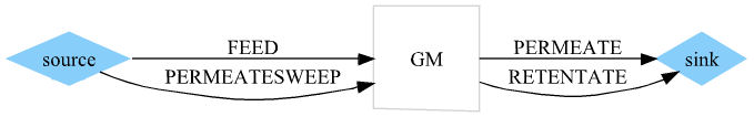
Connections:
-
netin i.e.
in1 -
permin i.e.
in2 -
netout i.e.
out1 -
permout i.e.
out2
as depicted in the following figure:
Input variables related to the MultiExchanger model:
A |
Active area of the membrane and for heat transfer | |
Input variables specific to the Membrane22Rtsc model:
permeance[n_c] |
Permeance of each component, corresponds to the variable |
|
deltaPretentate |
Retentate side pressure drop | Pa |
deltaPpermeate |
Pressure drop permeate side | Pa |
Explicit equations:
delta = (*inlets_[0]->Q("P") - deltaPretentate/2.0) / (*inlets_[1]->Q("P") - deltaPpermeate/2.0);
for (int i=0; i < NCOMPONENTS; ++i) {
  permeationFactor[i] = permeance[i]*A*(*inlets_[1]->Q("P") - deltaPpermeate/2.0)/N;
  lambda[i] = (*inlets_[1]->Q("Tphase.ndotcomps", i) + *inlets_[0]->Q("Tphase.ndotcomps", i)) / N;
  mrt_->theta[i] = (N * permeationFactor[i] * (delta * *inlets_[0]->Q("Tphase.x", i) - *inlets_[1]->Q("Tphase.x", i)) +
*inlets_[1]->Q("Tphase.ndotcomps", i)) / (*inlets_[0]->Q("Tphase.ndotcomps", i) + *inlets_[1]->Q("Tphase.ndotcomps",
i));
} // for each component
for (int j = 0; j < NCOMPONENTS; j++) {
  phases[1].ndotcomps[j] = outp[0]->flow(j) * theta[j] + outp[1]->flow(j) * (theta[j] - One);
  phases[0].ndotcomps[j] = -phases[1].ndotcomps[j];
} // for each component j
stageCut.clear();
for (int i = 0; i < NCOMPONENTS; i++) {
  stageCut += lambda[i] * mrt_->theta[i];
} // for each component
Results related to MultiReactionTransfer model:
multiReactions[0] = theta[n_c] |
Vector of stage cuts of each component, corresponds to the stage-cut of the single component |
- |
Results specific to the Membrane22Rtsc model: |
Tavg |
Average inlet temperature based on the average on a molar basis between permeate and retentate | K |
stageCut |
corresponds to the variable |
- |
delta |
Pressure ratio, corresponds to the variable |
Pa/Pa |
N |
Total molar flow rate of the two feeds | kmol/s |
permeationFactor[n_c] |
Permeation factor of each component, corresponds to the variable |
- |
lambda[n_c] |
Average molar fractions of the two feeds | kmol/kmol |
Membrane22Linear
Unit with two-two connectivity and global linear fluid dynamics.
It is very similar to the previous Membrane22Rtsc, from which it differs because the equations are not completely explicit and it is therefore necessary to solve iteratively for the variable
Results specific to the Membrane22Linear model:
stageCutEst |
estimated stage cut, corresponds to the initial estimate for the variable |
- |
The explicit equations differ only in the calculation of the stage-cut of the single component
mrt_->theta[i] = (lambda[i] + *inlets_[0]->Q("Tphase.x", i) * (One-stageCutEst)- (One-stageCutEst) *
*inlets_[1]->Q("Tphase.x", i) / delta + 2.0 * *inlets_[1]->Q("Tphase.ndot") * *inlets_[1]->Q("Tphase.x", i)
*(One-stageCutEst) / (N * permeationFactor[i] * delta)) / ((((One-stageCutEst) / delta) * (Quantity(2.0) /
permeationFactor[i] + One / stageCutEst) + One) * lambda[i]);
which is based on equation (36) from the additional theoretical annex.
Implicit equation: stageCutEst - stageCut = 0.
Full flowsheets
An actual process model is created with LIBPF® by writing 4 sections of highly-simplifed C++ code, resembling a Domain-Specific Language (DSL):
-
Define the units (using the low-level models described above):
makeVertex<MembraneMulti12<Membrane12Cstr> >("MODULE1", "Gas membrane unit 1", options); makeVertex<MembraneMulti12<Membrane12Cstr> >("MODULE2", "Gas membrane unit 2", options); makeVertex<Compressor>("C1", "Compressor 1", options); makeVertex<Compressor>("C2", "Compressor 2", options); makeVertex<Mixer>("MIX", "Retentate mixer", options); -
Define the connectivity (the streams connecting the units):
makeEdge<StreamVapor>("FEED", "System feed", "source", "out", "C1", "in", options); makeEdge<StreamVapor>("FEED1", "Membrane 1 feed", "C1", "out", "MODULE1", "feed", options); makeEdge<StreamVapor>("PERMEATE1", "Permeate from membrane 1", "MODULE1", "permeate", "C2", "in", options); makeEdge<StreamVapor>("RETENTATE1", "Retentate from membrane 1", "MODULE1", "retentate", "MIX", "in", options); makeEdge<StreamVapor>("FEED2", "Membrane 2 feed", "C2", "out", "MODULE2", "feed", options); makeEdge<StreamVapor>("PERMEATE2", "Permeate from membrane 2", "MODULE2", "permeate", "sink", "in", options); makeEdge<StreamVapor>("RETENTATE2", "Retentate from membrane 2", "MODULE2", "retentate", "MIX", "in", options); makeEdge<StreamVapor>("RETENTATES", "Total retentate from membranes 1 and 2", "MIX", "out", "sink", "in", options); -
Set feed flow, composition and conditions:
Q("FEED.P")->set(1.2, "bar"); Q("FEED.T")->set(40.0+273.15, "K"); S("FEED.flowoption")->set("Nx"); Q("FEED:Tphase.ndot")->set(1000.0/3600.0/22.7107836, "kmol/s"); my_cast<Stream *>(O("FEED"), CURRENT_FUNCTION)->clearcomposition(); Q("FEED:Tphase.x", "CH4")->set(0.65); Q("FEED:Tphase.x", "CO2")->set(0.35); Q("FEED:Tphase.x", "H2O")->set(0.0); -
Set the operating conditions of the units:
Q("MODULE1.permeance", 0)->set(100.0, "GPU"); // CO2
Q("MODULE1.permeance", 1)->set(100.0/30.0, "GPU"); // methane
Q("MODULE1.permeance", 2)->set(150.0, "GPU"); // H2O
Q("MODULE1.permeance", 3)->set(100.0/50.0, "GPU"); // N2
Q("MODULE1.Ppermeate")->set(1.0, "bar");
Q("MODULE1.A")->set(150.0, "m2");

...

Q("MODULE2.permeance", 0)->set(100.0, "GPU"); // CO2
Q("MODULE2.permeance", 1)->set(100.0/30.0, "GPU"); // methane
Q("MODULE2.permeance", 2)->set(150.0, "GPU"); // H2O
Q("MODULE2.permeance", 3)->set(100.0/50.0, "GPU"); // N2
Q("MODULE2.Ppermeate")->set(1.0, "bar");
Q("MODULE2.A")->set(50.0, "m2");

...

S("C1.option")->set("P");
Q("C1.P")->set(40.0, "bar");
Q("C1.theta")->set(0.75);
Q("C1.etaM")->set(0.95);
Q("C1.etaE")->set(0.98);

...

S("C2.option")->set("P");
Q("C2.P")->set(40.0, "bar");
Q("C2.theta")->set(0.75);
Q("C2.etaM")->set(0.95);
Q("C2.etaE")->set(0.98);
Merkel2010Fig7a and Merkel2010Fig7aLinearCounterflow: single-stage case for post-combustion
This is a post-combustion CO2 capture process for power plants based on reference [Merkel2010], Figure 7a:

According to the authors, their results are for counterflow without permeate sweep; two models of this separation system were developed to compare the results:
-
Merkel2010Fig7awith free flow membrane model with CSTR mixing -
Merkel2010Fig7aLinearCounterflowwith linear averaging counterflow model.
The main input data are shown in the table:
| Quantities | Value |
|---|---|
| 20,514 kmol s-1 | |
| 0,13 | |
| 1,1 / 1,0 bar | |
| 0,27 / 0,22 bar | |
| A | 6,8 · |
| 1000 GPU | |
| 20 GPU | |
Missing data were qualified as follows:
-
Inlet temperature 20°C
-
Inlet volumetric flow rate considered at inlet T and P conditions
-
Retentate side pressure drop 100 hPa
-
Permeate side pressure drop 50 hPa.
The results:
| Quantities | Paper results | LIBPF® Merkel2010Fig7a (free flow) results |
LIBPF® Merkel2010Fig7a LinearCounterflow results |
|---|---|---|---|
| x[CO2] | 2.1 % | 5.6 % | 2,1% |
| y[CO2] | 40.6 % | 33.5 % | 39.4 % |
| Compressor power consumption | 7.2 MW | 7.41 MW | 7.41 MW |
| Vacuum pump power consumption | 38.8 MW | 33.0 MW | 38.8 MW |
| Total power consumption | 46 MW | 40.4 MW | 46.2 M |
The countercurrent linear-averaged model satisfactorily reproduces the reference data. The free flow model has significantly worse performance (particularly relative to recovery).
Merkel2010Fig7bLinearCounterflow: Single-stage flow case with permeate sweep for post-combustion
This is a post-combustion CO2 capture process for power plants based on reference [Merkel2010], Figure 7b:

According to the authors, their results are for countercurrent flow with permeate sweep; to compare the results, a version of this module was made: Merkel2010Fig7bLinearCounterflow with countercurrent linear averaging model.
The main input data are shown in the table:
| Quantities | Value |
|---|---|
| 20,514 kmol s-1 | |
| 0,13 | |
| 1,1 / 1,0 bar | |
| 0,27 / 0,22 bar | |
| A | 4,3 · |
| 1000 GPU | |
| 20 GPU | |
Missing data were qualified as in the previous case.
The results:
| Quantities | Paper results | LIBPF® results |
|---|---|---|
| x[CO2] | 2,1 % | 2,5 % |
| y[CO2] | 40,6 % | 39,4 % |
| Compressor power consumption | 7,2 MW | 7,36 MW |
| Vacuum pump power consumption | 38,8 MW | 37,8 MW |
| Total power consumption | 46 MW | 45,14 MW |
As in the previous case, the results differed marginally from those reported in the reference.
Merkel2010Fig11: Three-stage case for post-combustion
This is a a three-stage plant for separating CO2 from N2 based on reference [Merkel2010], Figure 11:

The plant consists of two stages in series with recycling by means of which
In the flowsheet Merkel2010Fig11, the free flow model with global fluid dynamics CSTR MembraneMulti12<Membrane12Cstr> was used for the three membrane units, without considering the upstream part of the first compressor, i.e., coal combustion and particulate removal.
The main input data are shown in the table:
| Quantities | Value |
|---|---|
| 20,514 kmol s-1 | |
| 11,6 % | |
| 73 % | |
| 4,4% | |
| 11 % | |
| A | 3,6 · |
| 1000 GPU | |
| 50 | |
Missing data were qualified as follows:
-
Inlet temperature 20°C
-
Inlet volumetric flow rate considered at the conditions of inlet T and P
-
C1, C2 and C3 three-stage vacuum compressors and pumps, thermodynamic efficiency = 80 40°C
-
C1 discharge pressure 220 kPa
-
Retentate side pressure drop 100 hPa
-
Permeate side pressure drop 50 hPa
-
Permeance of water 20000 GPU
-
Surface area distribution among the three modules: GM1 35%, GM2 65% and GM3 0.03%.
The key results:
| Quantities | Paper results | LIBPF® results |
|---|---|---|
| 1,8% | 1,91% | |
| 50% | 50,6% | |
| 29% | 18% | |
| 24% | 22,4% | |
| 70% | 61,7% | |
| Recovery |
90% | 88,5% |
| Purity |
95% | 97,8% |
| Total power consumption for compressions |
131 MW | 161 M |
In this case the matching is imperfect despite attempts to optimize compressor efficiencies. The publication seems to promote this technology as more attractive.
Deng2010Fig6b: Dual-stage case for biogas upgrading with facilitated transport membranes
This is a complete two-stage plant for biogas upgrading with facilitated transport membranes (hollow fiber geometry), without recycle, taken from Figure 6b of [Deng2010]:

It should be emphasized that for transport-facilitated membranes it is not physically correct to apply equation (5) from the additional theoretical annex, which can be considered valid only in the sense of a linearization in a certain range of operating conditions; however, the case was treated because of the application interest.
In the flowsheet Deng2010Fig6b, the free flow model with global fluid dynamics CSTR MembraneMulti12<Membrane12Cstr> was used for the two membrane units, whereas in the reference a counterflow model implemented in the in-house simulation tool ChemBrane integrated within a commmercial process simulation environment was used; this tool has the special feature of calculating fluid properties with a cubic equation of state.
The main input data are shown in the table:
| Quantities | Value |
|---|---|
| 1000 = 0,01223 kmol/s |
|
| 0,35 | |
| 0,65 | |
| 1,2 bar | |
| 20 bar | |
| A | 1167 |
| 100 GPU | |
| 3,33 GPU | |
Missing data were qualified as follows:
-
C1 and C2 three-stage compressors and vacuum pumps, refrigeration temperature between compressor stages 40°C
-
Retentate side pressure drop 0 hPa
-
Permeate side pressure drop 0 hPa
The key results:
| Quantities | Paper results | LIBPF® results |
|---|---|---|
| Purity methane | 98 % | 98,0 % |
| Recovery methane | 97,3 % | 95,2 % |
| Total power consumption for compressions |
220 kW | 217 k |
Makaruk2010Fig2FreeFlowRtsc and Makaruk2010Fig2FreeFlowCstr: Dual-stage case for biogas upgrading
This is a two-step, low-pressure-feed biogas upgrading process with recycke, based on Figure 2 of [Makaruk2010]:

Two versions of this model were made both in free-flow, one with “RTSC” mixing (Makaruk2010Fig2FreeFlowRtsc) and the other with CSTR mixing (Makaruk2010Fig2FreeFlowCstr).
The main input data are shown in the table:
| Quantities | Value |
|---|---|
| 1000 = 0,01223 kmol/s |
|
| 0,4 | |
| 0,6 | |
| 1 bar | |
| 10 bar | |
| A | 2800 |
| Area ratio = = |
4 |
| 100 GPU | |
| 35 | |
The key results:
| Quantities | Paper results | LIBPF® Makaruk2010Fig2 FreeFlow Rtsc results |
LIBPF® Makaruk2010Fig2 FreeFlow Ctsc results |
|---|---|---|---|
| Purity methane | 98 % | 98,6 % | 97,1 % |
| Recovery methane | 98 % | 95,3 % | 95,2 % |
| Total power consumption for compressions |
160 kW | 155 kW | 157 k |

The resulting graph reflects the trend and values of the similar one in the reference:

Convergence for selectivity of 10 could not be achieved.
The results of LIBPF® model are only slightly worse at the nominal point, while there is a strong discrepancy for low recovery values and specific consumption at high area ratios. The latter could be due to different assumptions regarding compressor modeling.
Benchmark: conventional biomethane-to-electricity conversion process
This is a conventional technology for local power generation where raw anaerobic biogas is fed to an internal combustion engine (ICE):
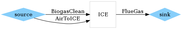
The plant size is set equal of the rated power of 1 MW ([Monteleone2011]).
Battery limits:
-
Ambient pressure: 1 atm.
-
Ambient temperature: 20°C.
-
Biogas temperature: 40°C.
-
pgraded methane delivery pressure equal to 2500 kPa g.
-
Biogas admission pressure from digester equal to 20 kPa g.
-
Biogas admission pressure to the internal combustion engine equal to 20 kPa g.
-
Specifications of upgraded biogas:
-
dew-point of water -5°C @ 7000 kPa g equivalent to 60 ppm v/v
-
< 3% v/v
-
The raw biogas stream from the digester is defined as follows:
| Quantities | Value |
|---|---|
| Molar flow rate | 530 |
| Molar fraction |
55 % |
| Molar fraction |
40 % |
| Molar fraction |
5 % |
| Pressure | 120 kPa |
| Temperature | 40 °C |
The assumed composition of atmospheric air is:
| Species | Molar fraction |
|---|---|
| 20,37 % | |
| 76,60 % | |
| 3.00 % | |
| 0.03 % | |
The air flow rate is set to maintain a residual oxygen mass fraction in FlueGas of 1%.
The available heat output is calculated assuming that flue gas is discharged to the atmosphere at a temperature of 80 °C.
The main results obtained characterizing the reference case are given in the following table:
| Quantities | Value | Unit of measurement | Description |
|---|---|---|---|
| LHVin | 2860.53 | kW | Heat input capacity based on Lower heating capacity |
| ICE:Wt | 2780.28 | kW | Heat output actually available (based on flue gas discharge temperature) |
| ICE:We | 973.099 | kW | Net electrical power generated |
| etaLhv | 34.1 % | Electrical output based on Lower heating capacity | |
Upgrading: Innovative upgrading process
The innovative biomethane upgrading is based on a two-stage medium-pressure process and bypasses a fraction of the raw biogas that is sent along with the permeate to the internal combustion engine:
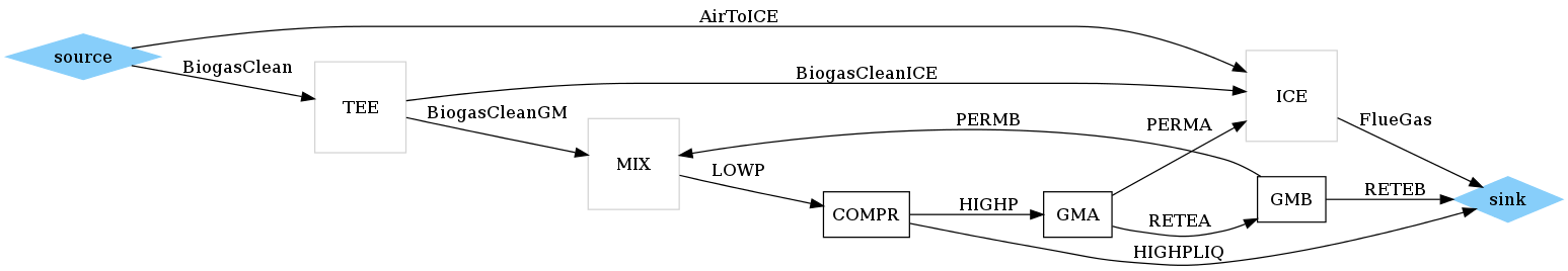
Battery limits are the same as for the Benchmark process.
To set the membrane properties, reasonable values were assumed although not supported to date by direct experimental measurements on an industrial scale.
For carbon dioxide permeance, the permeability values of [UniBo2011] at 3 bar pressure and 35°C temperature, converted to permeance based on a film thickness of 10
| Source | Membrane type | Permeance GPU | Permeance kmol/m2/s/Pa |
|---|---|---|---|
| [UniBo2011] | Matrimid | 19 | 6,1E-012 |
| [Yave2010] | thin film PEO-PBT | 120 | 7,3E-10 |
| [Merkel2010] | membrane MTR Polaris | 54 | 3,3E-10 |
| [Deng2010] | PVAm/PVA | 11 | 6,7E-11 |
Based on the reference [Merkel2010] and also based on the results for polymeric membranes made available by the partners [UniBo2011], a
For water permeance, it was assumed to be 150% of carbon dioxide permeance.
The key input parameters set were then:
| Quantities | Value | Unit of measurement | Description |
|---|---|---|---|
A |
250 | Total active area | |
Pin |
120 | kPa | Crude biogas pressure |
Pout |
2500 | kPa | Pressure of biogas after upgrading |
alpha |
35 | Selectivity |
|
areaRatio |
1 | Ratio between areas A2 & A1 | |
splitToIce |
0.2 | Fraction of raw biogas that bypasses the upgrading plant to proceed directly to ICE | |
COMPR.T |
313,15 | K | Intercooler temperature |
COMPR.etaE |
1 | Electrical efficiency for all stages | |
COMPR.etaM |
0.9 | Mechanical efficiency for all stadiums | |
COMPR.theta |
0.8 | Thermodynamic efficiency for all stages | |
GM{A,B}.deltaPretentate |
50000 | kPa | Retentate side pressure drop |
GM{A,B}.permeance[0] |
3,348· |
kmol m^-1 kg^-1 s | Permeance for |
GM{A,B}.permeance[2] |
5,022· |
kmol m^-1 kg^-1 s | Permeance for |
ICE.eta |
35 % | Electrical yield | |
The main results obtained are shown in the table below:
| Quantities | Value | Unit of measurement | Description |
|---|---|---|---|
LHVin |
2860 | kW | Thermal input power based on Lower heating capacity |
power |
131 | kW | Net electrical power generated |
powerConsumption |
73 | kW | Consumption per compressions |
powerProduced |
204 | kW | Gross Electrical Power Generated |
purity[0] |
2.19 % | Purity |
|
purity[1] |
97.79 % | Purity |
|
purity[2] |
0.02 % | Purity |
|
recoveryMembrane[0] |
2.82 % | Recovery |
|
recoveryMembrane[1] |
91.71 % | Recovery |
|
recoveryMembrane[2] |
0.25 % | Recovery |
|
recoveryTotal[0] |
2.25 % | Recovery |
|
recoveryTotal[1] |
73.37 % | Recovery |
|
recoveryTotal[2] |
0.20 % | Recovery |
|
Note how the mole fraction of water in the upgraded methane (243 ppm v/v) does not meet the specification on water (60 ppm v/v), in contrast, the specification on carbon dioxide is met.
Key performance indicators (KPIs)
The performance of the biogas upgrading process was evaluated based on the standard KPIs proposed in [Turchetti2011]:
-
Recovery (
), can be read from the above table as: = recoveryTotal[1]= 73.37 %. -
Purity (
), can be read from the above table as: = purity[1]= 97.79 %. -
Normalized specific energy consumption ($\mathcal{E}), can be obtained from the above table as:
= powerConsumption / (LHVin * recoveryTotal[1])= 3.48%
Clearly, an upgrading process can be designed or rather exercised in different ways, either by favoring purity at the expense of recovery or by maximizing both at the expense of specific energy consumption. The performance parameters proposed in [Turchetti2011] are therefore primary parameters in the sense that they can be subject to trade-offs in one direction or the other.
The performance parameter proposed in [Greppi2011b] attempts to further summarize performance, by defining a secondary parameter that allows comparison between processes set according to different criteria, referring to the benchmark process. This parameter is the Relative Power Gain on an electric basis (
The calculation of
where:
etaRemote = 55% |
efficiency of a remote thermal power plant with best-of-class |
Benchmark.etaLhv = 35% |
efficiency of internal combustion engine |
Premote = Upgrading.LHVin * Upgrading.recoveryTotal[1] * etaRemote |
electricity produced from upgraded methane in the remote thermal power plant |
Plocal = Upgrading.power |
Locally generated electricity, net of the electricity required to operate the separation plant |
Plocal0 = Upgrading.LHVin * Benchmark.etaLhv |
electricity that would have been produced locally in any case by the biogas in the internal combustion engine if it had not been upgraded |
Substituting the values gives:
References
Gas Membrane demo
-
This document is based on public-founded research activities performed in collboration with the Process Engineering Research Team of the Department of Civil, Environmental and Architectural Engineering of University of Genoa, Italy in the framework of the 2008-2009 “Ricerca di Sistema Elettrico”, project 2.1.2 (“Studies on local power generation from biomass and wastes”), objective C (“Development of processes and systems for biogas upgrading”), sub-objective C.1 (“State of the art analysis of processes to for CO2 removal from biogas”). See the other project deliverables on the dedicated area on the website of ENEA (the Italian National Agency for New Technologies, Energy and the Sustainable economic development).
LIBPF® technology
Scientific publications
[Deng2010] Liyuan Deng, May-Britt Hägg, Techno-economic evaluation of biogas upgrading process using CO2 facilitated transport membrane, International Journal of Greenhouse Gas Control 4 (2010) 638–646, doi: https://dx.doi.org/10.1016/j.ijggc.2009.12.013
[Greppi2011b] P. Greppi, E. Arato, B. Bosio, Rapporto PERT2 “Proposta di una metodologia di confronto delle tecnologie”, Marzo 2011
[Makaruk2010] A. Makaruk, M. Miltner, M. Harasek, Membrane biogas upgrading processes for the production of natural gas substitute, Separation and Purification Technology 74 (2010) 83–92, doi: https://dx.doi.org/10.1016/j.seppur.2010.05.010
[Merkel2010] Tim C. Merkel, Haiqing Lin, Xiaotong Wei, Richard Baker, Power plant post-combustion carbon dioxide capture: An opportunity for membranes, Journal of Membrane Science 359 (2010) 126–139, doi: https://dx.doi.org/10.1016/j.memsci.2009.10.041
[Monteleone2011] Giulia Monteleone, Caratteristiche richieste dal sistema di arricchimento in gas metano del biogas, Gennaio 2011
[Turchetti2011] L. Turchetti, M.C. Annesini, “Stato dell’arte sui processi di upgrading del biogas non basati su operazioni con membrane”, Marzo 2011
[UniBo2011] Risultati sperimentali relativi alle membrane in Matrimid, 2 Agosto 2011
[Yave2010] Wilfredo Yave, Anja Car, Jan Wind and Klaus-Viktor Peinemann, Nanometric thin film membranes manufactured on square meter scale: ultra-thin films for CO2 capture, Nanotechnology 2010,Volume 21, Number 39, doi: https://dx.doi.org/10.1088/0957-4484/21/39/395301